
EMI Debugging: If You Can See It, You Can Fix It
If you are a novice designer of electronic circuits, this is one of the best pieces of advice I can give you from my experience in EMI troubleshooting and training.
If you can see it, you can fix it. I am not sure who the author is of this sentence, but I really love it. In EMI/EMC, and electronic troubleshooting in general, to see the problem is a key to avoid the trial and error processes.
Your circuit is not working as expected; the system fails during an ESD test; or radiated emissions tests fail at some parasitic frequency of your design. The list of problems is infinite. But, for any of those problems, an effective solution is possible if you can find and see the signals involved in the failure.
1) The Most Effective Domain
First, think about the most effective domain for your view: time or frequency domain.
You will find time domain useful to detect glitches, ringing, periodic anomalies, synchronized events, etc. Frequency domain is the domain for the results when testing for EMC or evaluation of EMC components, filters, shields, etc.; and it is useful for filtering, demodulation, and other techniques.
My recommendation is clear: use both of them!
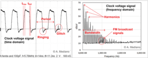
In Figure 1 (left) you see a digital clock in time domain. Ringing, period and rise-fall times can be easily measured. The spectrum of the signal is included in Figure 1 (right) where you can see the bandwidth of your signal. Amplitudes in both domains are related and rise/fall times impose the maximum frequencies in the frequency domain.
An oscilloscope is the typical instrument to use when interested in time domain. Usually, the alternative for the frequency domain is the spectrum analyzer, and sometimes scopes with FFT, but the use of FFT in scopes has been traditionally complex for novice users because of the need to set the time per division scales in the appropriate way to see the desired frequency range.
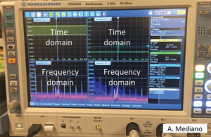
Today, you will find scopes (Figure 2) with powerful real time FFT, high bandwidth and trigger capabilities in the frequency domain, where FFT can be configured with the more common functions of CENTER FREQUENCY-SPAN or START-STOP FREQUENCIES. Limits are only in your mind.
2) The Adequate Probe
Now, you need to choose some variable(s) of your system to understand the behavior of the circuit under failure conditions. The variables can be chosen with two points of view: circuit theory with voltage (V) or current (I) or field theory with electric (E) or magnetic field (H). In this article I am not considering other variables such as temperature, audible noise, etc. for simplicity.
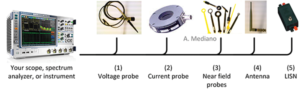
The variables from your selection determine the kind of probes you will need: voltage probes, current probes, antennas, LISN and near field probes.
Voltage probes: You will be able to see voltages in your analog or digital signals looking for periodicity, glitches, ringing, etc. This is the most common probe used by designers.
Current probes: Current probes are useful to measure current in traces and wires. Remember to consider if you are interested in measuring differential or common mode currents especially in cables.
Near field probes (NFPs): These probes are usually offered as small loops for magnetic fields or small tips for electric fields. NFPs are really useful to locate EMI sources, to inject EMI looking for susceptible circuits, or to analyze current paths
(i.e. decoupling evaluation).
Antennas: The transducers used to see electromagnetic field from far field sources.
Line impedance stabilization networks (LISN): This antenna is the way to measure or inject EMI in circuits through a conducted path (usually power supply) where load impedance must be known.
3) How Many Variables To See
Sometimes a mix of those variables and probes is the correct selection. For example, it is great to see how is common-mode current in your cable in frequency domain while you are looking at the magnetic field around a diode in the time domain (ringing).
The number of variables you will need determine how many channels you need in your instrumentation, especially when those variables must be observed at the same moment.
4) A Really Effective Tool
In recent years, near field scanners have been introduced in the market to measure in real time the activity of your design, to find EMI sources, to evaluate solutions, or to detect susceptible paths in your circuits.
As an example, in Figure 4, I have included the scan of a small PCB board with the EMxpert scanner from EMSCAN in my lab. With the experiment, we can see the effect of a series ferrite in a signal path.
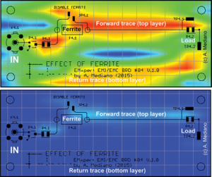
Note in upper part of the figure how the forward and return paths of the signal are clearly seen when the ferrite is not present and a big loop is present. In the lower part of figure the activity in the board is clearly reduced when the ferrite is present. The ferrite is effective and the current return paths are clearly identified.